Quick start

Info

You should be familiar with the command line, the QuPath core concepts and some basic Python know-how. Otherwise, you might want to check-out the full installation guide.

Installation

1. Install QuPath, ABBA and conda.
2. Create an environment :

   conda create -c conda-forge -n cuisto-env python=3.12
   

3. Activate it :

   conda activate cuisto-env
   

4. Install cuisto

   pip install cuisto
   

   If you want to build the doc locally :

   pip install cuisto[doc]
   

Data preparation

There are some required steps to take with the data prior to use cuisto for final results. You can find a prerequisites checklist here. There is also a pipeline that you can follow beforehand : this will handle the various files locations and related paths used by cuisto so it is easier to use afterwards.

The process of preparing the data before analysis is the following :

1. Acquire some imaging data
2. Make sure the images are pyramidal
3. Create a QuPath project
4. Use ABBA to register your slices on a reference brain atlas to get brain regions (so called Annotations). Alternatively, draw custom Annotations directly within QuPath -- make they sure they are formatted as expected by cuisto
5. Find objets of interests (so called Detections) in your slices with QuPath
6. Add measurements to those annotations : objects count, cumulated length, ... Atlas coordinates can also be added to the detections measurements to compute and plot spatial distributions.
7. Export the data from QuPath

Usage

Once you have a bunch of pairs of CSV files (one for annotations, one for detections), you can use cuisto to collate the data, derive quantifying metrics and spatial distrubutions and plot the results in a configurable manner. You'll need a configuration file, a text file easily editable to match your needs.

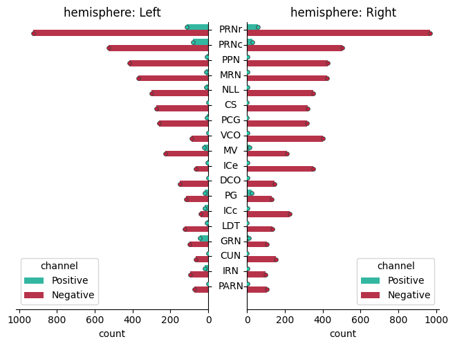
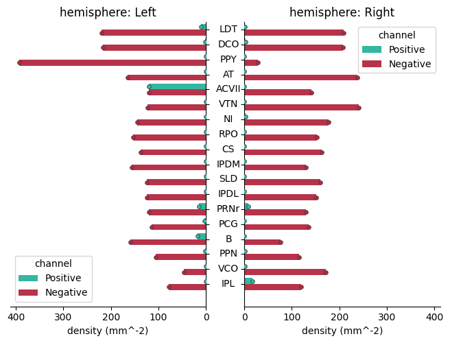
Two types of cells detected in a single animal

Gather data, compute metrics :

import cuisto
import pandas as pd

animal = "animal_id"

# files paths
config_file = "/path/to/config.toml"
annotations_file = "/path/to/annotations.tsv"
detections_file = "/path/to/detections.tsv"

# read configuration and data
cfg = cuisto.config(config_file)
df_annotations = pd.read_csv(annotations_file, sep="\t")
df_detections = pd.read_csv(detections_file, sep="\t")

# pool brain regions from different slices, compute density and spatial distributions
df_regions, dfs_distributions, df_coordinates = cuisto.process.process_animal(
    animal, df_annotations, df_detections, cfg, compute_distributions=True
)

Display raw object count and density per regions :

cuisto.display.plot_regions(df_regions, cfg)

Display spatial distributions (pdf) along the three axes :

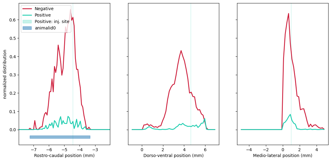
Check the full example notebook here.

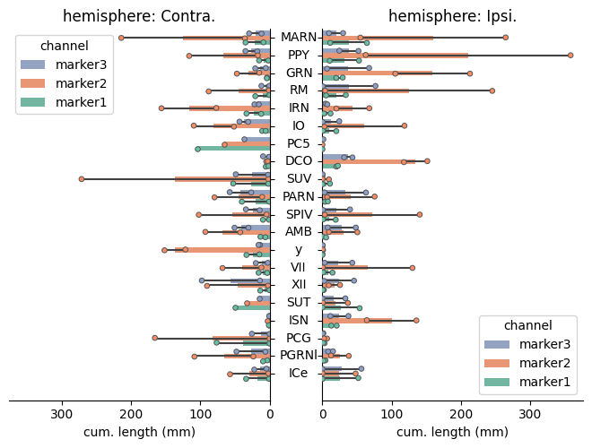
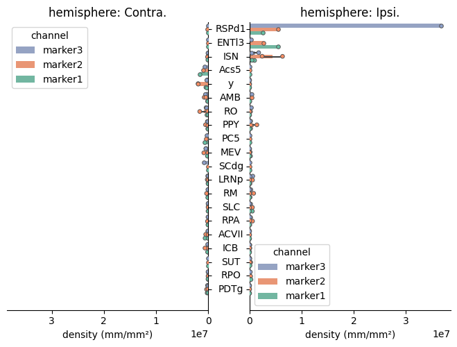
Axons with three staining from two animals

This dataset was analyzed fulfilling the pipeline requirements : some_directory contains a folder per animal.

import cuisto

# Parameters
wdir = "/path/to/some_directory"
animals = ["AnimalID0", "AnimalID1"]
config_file = "/path/to/your/config.toml"
output_format = "h5"  # to save the quantification values as hdf5 file

# Processing
cfg = cuisto.Config(config_file)
df_regions, _, _ = cuisto.process.process_animals(
    wdir, animals, cfg, out_fmt=output_format
)

# Display
cuisto.display.plot_regions(df_regions, cfg)

Check the full example notebook here.